Introduction

By reading this post, I hope that you will gain an intuitive understanding of adversarial examples. They are not as spooky and magical as they appear at first, and maybe it isn't even surprising that they exist. First, I will quickly cover what I mean by adversarial images. Second, I will discuss ImageNet classifiers. Finally I will use a two-dimensional example build an intuitive understanding.

What are adversarial images?

An adversarial example is a data point that has been manipulated by an adversary with some goal in mind, probably a goal opposite to yours. In the case of an image classifier, it is a natural image, that has been modified by an adversary in order to fool the classifier. The goal is typically either to get the classifier to output a specific class rather than the correct class (a targeted attack) or simply to get the classifier to output the wrong class (a non-targeted attack).

Fairly recently, everyone was quite surprised to discover that you can easily fool Deep Neural Networks (DNNs) with a very small change to an image. These are changes that a human would not even perceive. We are faced with the possibility that deployed classifiers in the real world could be fooled by an adversary when a human supervisor would not even realize what is happening. For any application with a potential adversary this is a problem, and for any application where there are safety considerations this is a big problem. A surveillance system could be fooled into ignoring exactly the bad people it is looking for. A virus scanner could be similarly challenged. What if pranksters fool our self-driving cars into identifying stop signs as yield signs? The consequences could be tragic.

Publications on the topic are littered with same-looking images with captions that claim they are classified differently by a classifier.

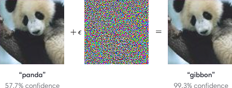
Figure: An example from the people at OpenAI

This is an academic field with real world importance, but I haven't yet seen any well articulated attack scenarios. This means that we tend to speak generally about an adversary changing the input to our classifier without specifying how they did it or what their limitations were. If an adversary can change every pixel of the image to whatever they want, it's little surprise that they can fool a classifier. They could simply substitute any image they like. Therefore it only makes sense to talk about adversarial examples in the context of small changes. Typically you either try to fool a classifier while minimizing the change, or alternatively you try to fool it as much as possible within some constraint as to how large the change is allowed to be.

What are ImageNet classifiers doing?

For simplicity, we will talk about the generation of models that take RGB images with width and height both 299 pixels as inputs.

Neural networks generally, and ImageNet classifiers in particular, are mapping vector spaces. An input image is just a collection of numbers, a red, green, and blue value for each pixel. An image can be thought of as \( 299*299*3 = 268203\) different variables, each taking a value in \([0,255]\). A single image can be thought of as a point in a 268,203-dimensional vector space. An ImageNet classifier is mapping that input space to a space of 1000 probabilities, one for each class. We train the classifier with training data to be a function that takes in any point in the input space and outputs a point in the output space. Given an image, here are the class probabilities.

Our training data is comprised of 1,000,000 natural images from the 1,000 classes. That is a lot of data and that is what makes training these neural networks possible. However, we know that this is actually only a tiny subset of all possible data. Imagine all possible photos of all possible instances of all possible ImageNet classes taken from all possible angles under all possible lighting conditions, and so on and so on. The number of possible images is clearly much much greater than the one million images in our training data. It would be tempting to conclude that the number is infinite, but we know that is actually not the case. Consider drawing randomly from the space of all possible 299x299x3 images. Set every pixel value randomly and study the result. How long would you expect to draw random images until you got one that looks like a normal photograph? I think probably all of humanity could perform this task for the rest of time without being successful.

So we are left with the conclusions that natural images make up a tiny proportion of our input vector space and that our training data makes up a tiny proportion of natural images. That means our classifier is learning to map a vector space that is mostly noisy garbage images, and it's learning to do that from actually very limited training data.

Where do adversarial images come from?

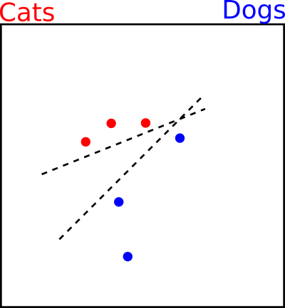
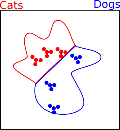
To build an intuition with visualization, we will consider an simplified two-dimensional example. No longer will we talk about 299 pixels by 299 pixels RGB images that define 260,203-dimensional vector spaces. Let's instead pretend that we have 2 pixels by 1 pixel gray scale images. They have only two pixels and only one value per pixel. Somehow imagine that it is possible to identify some of these tiny images as cats and some as dogs. We have six images in our training set (3 cats, 3 dogs), and since there are only two values, we can visualize them in a scatter plot. We will seek to train a classifier that can take in another of these strange images, and output a class of cat or dog.

Our two pixel images in a scatter plot:

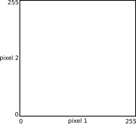
Our training set is six images. Three cats and three dogs. Each image has a different value for pixel 1 and for pixel 2. We are therefore able to plot these images in our scatter plot.

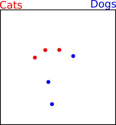
There is a true distribution of images that our training data comes from. It is impossible for us to ever know it, because we only have our training data points. Some regions are cats, some regions are dogs, and some regions are neither, perhaps just random meaningless images. I'll make up two hypothetical regions.

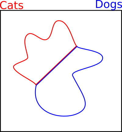
We use the training examples to train the classifier to draw a decision boundary between them. The boundary is a line where the probability of cat and dog are equal at 0.5, and on either side the decision is clear. We hope that when new test examples are drawn from somewhere in the red or blue areas, they will be classified correctly.

Unfortunately the training examples don't cover the space entirely, so there are a lot of different boundaries that could be drawn. This will always lead to errors at test time.

There are large areas with no training data that we don't care about at all. The neural network can do whatever it wants with the decision boundaries in this space. It's chaos for all we know.

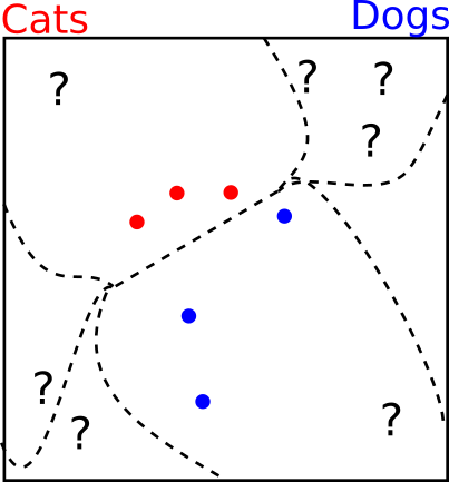
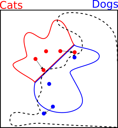
Consider the following decision boundary. It looks a little strange, but it correctly classifies the training data, does a decent job of covering the true space, and behaves weirdly in the empty space. It seems strange in our two dimensional case, but for larger images this is very plausible.

In the diagram below I use a black arrow to indicate an attack. We take a natural image from our training data, and then add or subtract a little from each of the two pixel values in order to move it into a different area of the scatter plot.

This gives us three ways of creating adversarial images by making small changes.

1. We move a cat from the region of true cats that were correctly classified, into a region where they are not.

2. We move a dog out of the region of natural images, and into the area where the decision boundaries are chaotic. We choose a place that is classified as cat.

3. We move a cat from the region of true cats into the region of true dogs, causing it to be misclassified. In theory this attack would work on a human because we literally changed the meaning of the image.

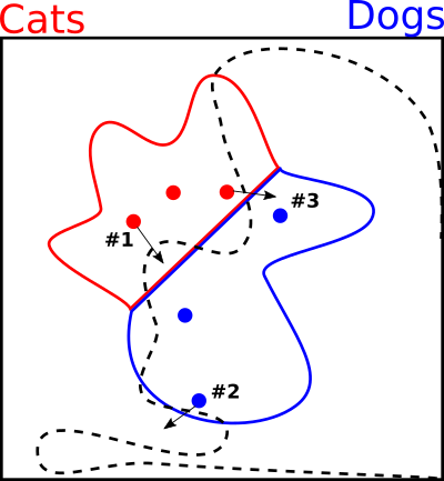
If the change is small enough, a human won't notice the difference.

When attackers are creating these adversarial images, they don't really know which of the three scenarios are occurring. If the attackers could know that, then so could the defenders and adversarial images wouldn't be a problem.

At the top of the article we had a panda changed into a gibbon. I think that we can agree this is an example of #1 above. The image is still a normal looking image of a panda, but it is misclassified.

Here's an interesting example of a natural image and an attacked image from Ben Hamner's kernel:

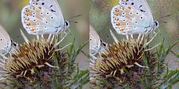
The attacked image on the right is still obviously a butterfly, but there's something odd about it. There's a bizarre noise pattern that would not occur in a normal image. This is an example of #2.

Finally here's something I created recently as part of a project:

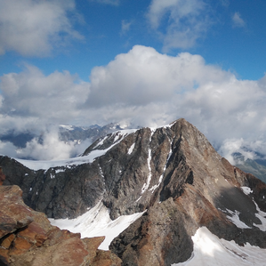
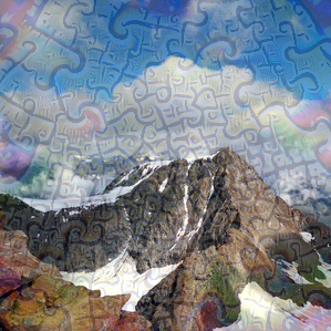
The goal was to get an ImageNet classifier to output something other than mountain, which it obviously is. The attacked mountain on the right has an unnatural quality to it, but to a human eye, it actually looks quite a lot like a jigsaw puzzle of a mountain, as was my intent. This is an example of #3. We have changed the true meaning of the image such that even a human might get it wrong.

What can we do to defend?

One of the most basic defenses is "adversarial training". Essentially we attack our own classifier and then add those examples as training data. Doing so allows us to pad the area around our training data so that decision boundaries are well behaved there, even though no "natural image" should ever appear there. This is effective to some extent, but with hundred of thousands of dimensions to cover, it seems hopeless that we'll ever be able to pad the entire space of natural images, let alone the space around our training data.

We add the examples from our three attacks above and re-train our classifier to get a new decision boundary.

As an aside, this is very similar to what we are doing when we do data augmentation. Using our prior knowledge about what transforms do not change the meaning of an image, we create more training data in the region of each image to help the classifier map the space.

Conclusion

So there you go. I hope this gives you an intuition for adversarial images and makes them a little less magical.